conditional formatting | chapter 2 | icon set | top 10 items | bottom 10 items

        Conditional Formatting Chapter 2 

 

Top Bottom Rules

Today we are going to understand several 'Top Bottom Rules'- 

Top 10 items: 

Under this rule excel highlights Top 10 items from your selected data range.

You can increase or decrease the basis of selection. For instance you can select top 5 from your selection.

How top 10 works?
Simple logic with unique values.

With unique values

But there is a trick when there are ties or duplicate values. Lets understand the logic with the help of a video.

 

Top 10% 

Explained with the help of an example below

Bottom 10 Items 

Similar to Top 10 items. Read above.

Sometime it is hardly possible to identify bottom 10 or top 10 values at a glance. 

Excel is absolutely smart in this matter. (Look below)

Bottom 10% 

Bottom 10% rule is also similar to the Top 10% rule as discussed above. Here instead of top values excel deals with lower values in the data range.

Above average and Below Average 

This two option works with simple logic. Just highlighting values above and below average.
We can combine the "above average" and "below average" in a same data range by changing the color of the respective highlights. In the display below we opted separate data range for easy understanding.

Above average and Below average

Data Bars 

 

Data bar options displays the data the data in a range by applying color gradient on the cell. It is sometimes visually pleasing. Without delving into the details we can at a glance understand the present status of the data in the order of comparison. Say small value gradient bar is light and small. High value gradient bar is dark and long. Gradient means gradual. Instead of gradient we can use solid fill.

Color Scales 

Color scales displays the transition of color between two values in comparison.


In the above display we can see lowest value of the range is 1028 and highest value 9979. And 1028 is pinned with solid Red and 9979 is highlighted with solid Green. Now observe the transition of colors of the remaining cells that falls within the two extreme points (1028 & 9979). If we observe very carefully not a single color is matching with any other color in the data range. Though the data range doesn't have any duplicates. If there are duplicates the color will match.

Icon Set 

 

In the Icon set function we will manage rules. That is we are going to customize the rules at our discretion. It is to be noted all the rules can be managed.
We will understand with the help of a video.

conditional formatting | Chapter 1 | greater than

                                   Conditional Formatting

 

In this topic we are going to excavate a very important and serious application of excel. We will understand how it works precisely.

                                     
                                         

After clicking conditional formatting button several options are available including sub options.

Highlight cells rules further categorized as

Greater than 

 

Under this function content of cells that are greater than a specified number are highlighted. After selecting the data set (A5 to C9) click Greater than option.

There are various highlighting option. We opted here 'Light Red fill with dark Red text". Highlighting option can be customized.

Excel has selected greater than 400 from the above data series. And the selected data are pinned with Red.In the Greater than window the Red circle indicates that by clicking on we can separately denote a cell containing the value greater than 400 instead of writing 400 in the space left.

Less Than 

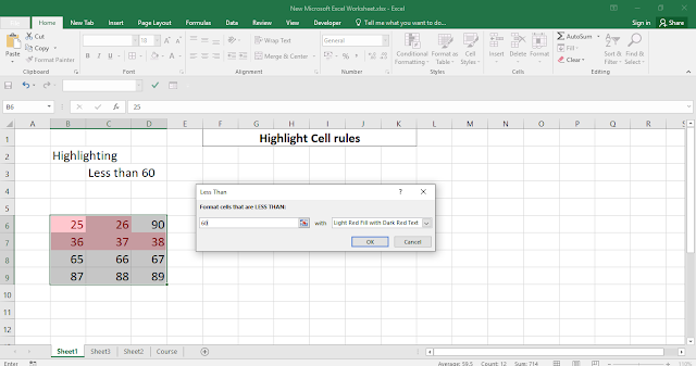
By clicking the Less than option under Conditional Formatting we are highlighting those values that are less than 60.

Between 

 

This option determines the values between two specified extremes. 

Highlighting values between 41 to 74. 

Equal to

Highlighting 25 only. 

Text That contains....... 

Lets understand this function with a help of a video.

A date occurring 

 

This format only works when you are working on the basis of the current month (when system date is the basis of the working date)
Since we are at this moment in the month of September 2019.
The video will help you to understand this format.

Duplicate values/Unique values 

This format is widely used among the conditional formatting option. We will fetch the duplicate values and unique values from our data range in the custom manner.Watch the video

Some important tips on duplicate values.

Similar values or text are highlighted under duplicate value format.
This format is sensitive. If two data looks apparently same, but one is followed by spaces then it will pinned those two as unique.It ignores uppercase & lowercase. Similar values with different cases (one is in upper case and another one in lower case) are pinned as duplicate values. 
Practice with your own data.