Pivot table | Chapter 3 | Value field setting

This post is the continuation of the immediate previous post.

A Simple data we are going to use in Field settings for Pivot table. You can copy this data in your Excel sheet and try.

 

Default Pivot table from above data

 

Field Setting 7

Lets deal with different standard deviation settings.

• Click inside the pivot table and activate Analyze tab. 
• Click 'Field settings', activate 'Summarize values by' tab if not activated. 
• Highlight the option 'Stddev'
• Click Ok 

Explanations:  

• In the Value Field settings four settings are found.
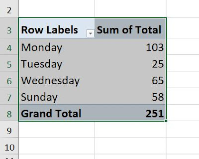
• In the Value Field settings in Pivot table these formulas are used namely stddev, stddevp, var, varp
• formula '=stddev(56,47)' results in 6.3639.... which is similar what Pivot Table adopts when we select Stddev from the list.
• In case of single digit there cannot be any deviation hence #Div/0!
• formula '=stddev(58,56,25,65,47)' results in 15.4822479. 
• Similarly with stddevp and others we can get the tabulated results in the pivot table.
• How formula works is outside the purview of this post.

   

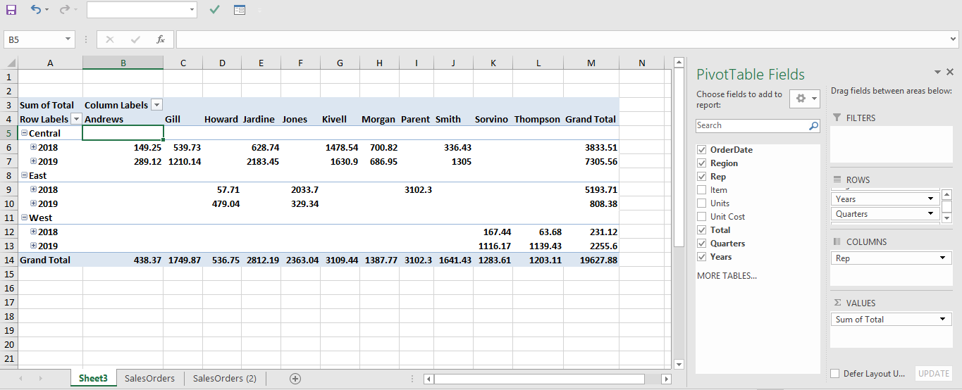
In the next instances we are going to use a different pivot table with little more data.

Download the datasheet
 

Pivot table from above data. 

 

Field Setting 8

Lets represent the above table on the basis of '% of grand total'.

• Click inside the pivot table and activate Analyze tab. 
• Click 'Field settings', activate 'Show values as' tab if not activated. 
• From the drop down menu 'Show values as'
• Highlight the option '% of Grand Total'
• Click Ok

Explanations:

• 100% Grand Total is the sum of (6.63+10.97+82.40)%
• Similarly 82.40% is the sum of 37.09%+45.30%

Field Setting 9

Lets represent the above table on the basis of '% of column total'.

• Click inside the pivot table and activate Analyze tab. 
• Click 'Field settings', activate 'Show values as' tab if not activated. 
• From the drop down menu 'Show values as'
• Highlight the option '% of Column Total'
• Click Ok

Explanations:

• All the column total is represented as 100%
• The performance of the representative 'Gill' in the Central region is 56.62% in 2018 and 43.38% in 2019. Say his performance declined in 2019.
• Grand total is same as before instance.

Field Setting 10

Lets represent the above table on the basis of '% of row total'.

• Click inside the pivot table and activate Analyze tab. 
• Click 'Field settings', activate 'Show values as' tab if not activated. 
• From the drop down menu 'Show values as'
• Highlight the option '% of Row Total'
• Click Ok

Explanations:

• All the row total is represented as 100 percent in the extreme right of the table.
• In case of Representative 'Andrews' his total performance on the basis of Central region is 3.44% where as his performance is 6.26% of the total performance in 2019.
• Sum total of all rows are 100%.

Field Setting 11

As it is apparent from the default pivot table that the Representative Smith's performance is the highest and best of the lot.

Lets present the above table on the basis of comparison of other representatives with Smith only.

• Click inside the pivot table and activate Analyze tab. 
• Click 'Field settings', activate 'Show values as' tab if not activated. 
• From the drop down menu 'Show values as'
• Highlight the option '% Of '
• Select Base field as Rep (Representative)
• Select Base Item as 'Smith'
• Click Ok

Explanations:

• I find this representation very logical.
• If we observe carefully we can see that representative Smith only performed in Central region in 2019. So comparison should be restricted to Central region for 2019.
• So Andrews, Gill & Jardine's performances are compared with Smith and represented in percentage format. Others are Null. 
• Similarly Central region's Sub Total is also compared on the basis of same logic. Only Kivell performance is compared and represented on the basis of Sub Total. Since Kivell and Smith performed in the same region.
• Only Smith performance is represented in 100 percent.

Field Setting 12

Lets represent the Pivot table on the basis of percentages of Parent row total.

Here parent row signifies sub total values at the top.

• Click inside the pivot table and activate Analyze tab. 
• Click 'Field settings', activate 'Show values as' tab if not activated. 
• From the drop down menu 'Show values as'
• Highlight the option '% of Parent Row Total '
• Click Ok

Explanations:

• Where there are performances the sub total is considered as 100% (all marked with Red)
• Say 56.62% and 43.38% together comprises 100%
• Grand Total is compared on the basis of 4634.03 data.
• Say 6.63% (As active Cell) arrives from dividing 307.37 by 4634.03 multiplied by 100, similarly 10.97% and 82.40% arrives in the same manner.

Field Setting 13

Lets represent the Default Pivot table data as 'Percentages of Parent Column Total'.

• Click inside the pivot table and activate Analyze tab. 
• Click 'Field settings', activate 'Show values as' tab if not activated. 
• From the drop down menu 'Show values as'
• Highlight the option '% of Parent Column Total '
• Click Ok

Explanations:

• All the cells of the Grand Total column is marked as 100%
• Performances are measured on the basis of Grand Total Value.
• All the percentages total of any row is 100%
• Even total of Grand Total row is 100%
• All row totals are 100%

Field setting 14 

Lets represent the pivot data as percentage of parent total.

• Click inside the pivot table and activate Analyze tab. 
• Click 'Field settings', activate 'Show values as' tab if not activated. 
• From the drop down menu 'Show values as'
• Highlight the option '% of Parent Total'
• Select the Region as Base Field
• Click Ok

Explanations: 

• All the parents (Region totals for representatives) are presented as 100%.
• Data are represented in percentage.

Field Setting 15 

Lets represent all the representatives performance data as a difference from representative Andrews.

• Click inside the pivot table and activate Analyze tab. 
• Click 'Field settings', activate 'Show values as' tab if not activated. 
• From the drop down menu 'Show values as'.
• Highlight the option 'Difference From'.
• Select the 'Rep' as Base Field.
• Select 'Andrews' as Base Item.
• Click Ok

Explanations: 

• Andrews has performed in Central region only. And he was the worst performer. 
• There is no subtotal for Andrews in the Central Region.
• Gill's difference is (953.27-131.34) 821.93 similarly others are projected in the subtotal zone.
• Negative values has been rejected.

Field Settings 16 

 Lets represent all the representatives performance data as a difference from representative Andrews in percentage format.

• Click inside the pivot table and activate Analyze tab. 
• Click 'Field settings', activate 'Show values as' tab if not activated. 
• From the drop down menu 'Show values as'.
• Highlight the option '% Difference From'.
• Select the 'Rep' as Base Field.
• Select 'Andrews' as Base Item.
• Click Ok

Explanations: 

• Here Gill's difference in percentage format is 625.80% that is 821.93 (observe field setting 15) divided by 131.34 (Andrew's Performance) and multiplied by 100. That is 821.93/131.34*100 result is 625.80%

Field Settings 17

Lets represent all the representatives performance in running total mode.

• Click inside the pivot table and activate Analyze tab. 
• Click 'Field settings', activate 'Show values as' tab if not activated. 
• From the drop down menu 'Show values as'.
• Highlight the option 'Running Total in'.
• Select the 'Rep' as Base Field.
• Click Ok

 

Explanations: 

• Grand total column is hidden.
• Running total is total is easy presentation.
• Say in Central 131.34, 131.34+953.27=1084.61,1084.61+429.14=1513.75 so on

Field Settings 18 

Lets represent all the representative's performance in running total mode and in percentage format.

• Click inside the pivot table and activate Analyze tab. 
• Click 'Field settings', activate 'Show values as' tab if not activated. 
• From the drop down menu 'Show values as'.
• Highlight the option '% Running Total in'.
• Select the 'Rep' as Base Field.
• Click Ok

Explanations: 

• Observe the previous table under the head Field Settings 17.
• In the Central region Andrews performance is 3.44% - is the percentage of 131.34 of 3818.25. Similarly 28.41% - is the percentage of 1084.61 of 3818.25 and so on.

 

Field Settings 19 

Lets rank the performance of representatives from Smallest to Largest rather worst to best.

• Click inside the pivot table and activate Analyze tab. 
• Click 'Field settings', activate 'Show values as' tab if not activated. 
• From the drop down menu 'Show values as'.
• Highlight the option 'Rank Smallest to Largest'.
• Select the 'Rep' as Base Field.
• Click Ok

Explanations: 

•  Andrews is the worst performer ranked as One (since smallest to largest) under grand total.
• Smith is the best performer ranked as Seven (since smallest to largest) under grand total.

 

Field Setting 20 

 Lets rank the performance of representatives from largest to smallest rather best to worst.

• Click inside the pivot table and activate Analyze tab. 
• Click 'Field settings', activate 'Show values as' tab if not activated. 
• From the drop down menu 'Show values as'.
• Highlight the option 'Rank Largest to Smallest'.
• Select the 'Rep' as Base Field.
• Click Ok

Explanations:

• Representative Smith is the best performer and ranked as one in grand total.
• Representative Andrews is the worst performer of all and ranked as seventh in grand total row.

Field Setting 21 

Index setting

Calculation is as follows

(Value in Cells X Grandtotal of Grand Totals)/(Grand Row Total X Grand Column Total)

• Click inside the pivot table and activate Analyze tab. 
• Click 'Field settings', activate 'Show values as' tab if not activated. 
• From the drop down menu 'Show values as'.
• Highlight the option 'Index'.
• Click Ok

Calculations for 

• 1.213652851 is (131.34 X 4634.03)/(3818.25 X 131.34)
• 2.207332641 is (131.34 X 4634.03)/(2099.38 X 131.34)
• If all value in the pivot table are equal each index will be 1
• If an index less than 1 it signifies that it is less important.
• If an index more than 1 it signifies that it is more important.
• Decimal places can be reduced.

Pivot Table | Chapter 2| Modifying pivot table

This post is the continuation of immediate previous post... 
One can download the data sheet (we are going to follow) from the previous post.

Instance 4

 Query: Representation of region wise sales of Rep (Representatives) on the basis of Date.

Pivot Table With Date field

• As we can see the Grand total is same as before. 
• The check box associated with Order date is checked. 
• Fields like 'Quarters' and 'Years' are generated automatically.
• Under Row area the fields like 'Years', 'Quarters' and 'Order Date' has been placed.

Another important thing can be noticed in the pivot table. Some +/- signs are visible in the table. Double clicking the + sign further disintegrates the data and table shows more precise information.

Modifying Pivot Table

The above table is without any subtotals. 

Modify 1

 Lets introduce sub totals.

• Click inside the Pivot table, Design tab activates.
• Click Subtotals (Extreme Left)
• Click 'Show all subtotals at the top of the group.

Sub Totals introduced at the top of the group

Explanation: 19627.88 is the sum total of 11139.07, 6002.09 and 2486.72. Similarly instead of pasting sub totals on the top you can paste it at the bottom of the groups. And you can also disable sub total.

Modify 2

Lets remove Grand Totals for Row and Column

• Click inside the pivot table.
• Under Design tab, click Grand Totals
• Click 'Off for Rows and Columns'

 

Modify 3 

By default all pivot tables are in Compact form. 

Reporting layout can be changed. 

Tabular Form

• Click inside the pivot table. 
• Under the Design Tab click Report Layout.
• Click 'Show in Tabular Form'.

This format is useful. 

Modify 4

Just to enhance the readability of the report we can introduce blank rows after each records.

  

• Click inside the pivot table.
• Under Design tab click Blank Rows.
• Click 'Insert Blank line after each item'.

 

Other modifications

 

Row headers, Column Headers, Banded rows, Banded columns and Pivot styles are self explanatory. One can use those at his or her 
discretion. 

Field Settings

We are about to dive deep into the pivot table's advanced features and functions.

One can get the dialogue box of Field Settings by right click on the pivot table and click 'Value Field Settings'.

With Field Settings we can modify the displayed data in the pivot table, of course without altering the source data.

For clear understanding we are going to use simple data. Logic is important.

Field Setting dialogue Box

• The Data is in Table Format
• In the Day field 'Monday' is repeated twice.

Default pivot table with Grand total of Total

Field Setting 1 

 Count the number of Data

• Click inside the pivot table and activate Analyze tab.
• Click 'Field settings'.
• Activate 'Summarize values by' tab if not activated.
• Highlight the option 'Count'
• Click Ok

Total Record Count

Explanation: 

• Monday is 2 (since repeated twice)
• Grand total 5

Field Setting 2 

Find the average of all records. (This is bit tricky)

• Click inside the pivot table and activate Analyze tab.
• Click 'Field settings'.
• Activate 'Summarize values by' tab if not activated.
• Highlight the option 'Average'
• Click Ok

Field settings Average

Field Setting 3 

Lets find the Maximum out of the field 

• Click inside the pivot table and activate Analyze tab.
• Click 'Field settings'.
• Activate 'Summarize values by' tab if not activated.
• Highlight the option 'Max'
• Click Ok 

Field setting Max

Explanations: 

• As per 'monday' record 56 is max 
• As per total record 65 is chosen as the maximum of all. 
• Row label is changed to 'Max of Total'.

Field Setting 4 

Finding the Minimum Value is similar to maximum value, rather the result is just the opposite.

Field Setting 5 

Lets find the product of all.

• Click inside the pivot table and activate Analyze tab.
• Click 'Field settings'.
• Activate 'Summarize values by' tab if not activated.
• Highlight the option 'Product'
• Click Ok 

Field setting Product

Explanations: 

• For Monday record the product of 56x47 is displayed.
• Grand total is the product of all records including 2632.

Field setting 6

Count the number of records.

For these data source 'Count' and 'Count numbers' are same.

Requires here no further explanation.

Pivot table | chapter 1 | Default Pivot Tables

Pivot Table

Pivot table is one of the most important feature of Microsoft Excel.
Endless rows and columns can be presented in a meaningful format.
Pivot table is the answer of endless queries. It is highly interactive, even after creation and presentation one can change it again.

Its a dynamic summary report from a database.

A simple shortcoming is, it cannot update itself automatically if there is a change in the source data.

A simple Pivot table set up

Download the sample data that we are going to deal with in this topic. click here

I think it is always better to convert the data source in excel table format first before arranging pivot table from the data source.
Excel will automatically update the pivot table in case a new data is introduced in the table.

In Pivot Table your source data should be in a rectangular database format. Informations that are available in the source should be of two types. 
Data (Say Total)
Data Category (Central Regions Total, even Smith performance total)

Default Pivot Tables

Instead of creating of pivot table from scratch one can select from some default styles provided in Excel. Under 'InsertTab' click 'Recommended Pivot Tables'. 

Excels provides some ready made Pivot Tables for your use. Intelligently it recognizes the data, one is dealing with.

• Select the entire Data range / click inside the range.
• Click Recommended Pivot Tables.

Recommended Pivot Tables

From here even you can start your own Pivot Table by clicking Blank Pivot table button.
The table above contains 7 columns.

1. Order Date
2. Region
3. Representative (Rep)
4. Item
5. Units
6. Unit Cost
7. Total (Unit x Unit Cost)

Highlight any option and click Ok the pivot table will be placed in a new sheet with Pivot Table fields.
Even you can start your own pivot table from this option.
Say we select 'Sum of total of Region' from the list

Sum Total of Regions

By default the table is placed in a new sheet.You can see the accuracy of the table, Grand Total confirms the sum of Total column. 

Lets modify the pivot table at your discretion.

This is to remember that one should start with a query for the presentation. There are innumerable queries, we will discuss few in this respect. One should practice with his own data set.

Laying out Pivot table

Fields in the 'Pivot Table Fields' window can be dragged in four spaces (Filter, Column, Row and Values). Say field 'Region' can be dragged in the Row area and field 'Total' can be dragged into the Value Space. Again if you want to remove any field from the above 4 spaces just drag out the field from the space. Or left click on the field on any of the 4 spaces, click 'Remove Field'.

Instance 1

Query: Presenting how Representatives performed in different regions.

• Click the check box relevant to Rep in Pivot Table Fields Task Pane.

 

A new tab 'Analyze' has been generated in the above ribbon. It is activated if we click anywhere inside the pivot table. As you can see in the above display a new field 'Rep' has been incorporated under Row option. 

Instance 2 

Query: Presenting how Representatives perform item wise in different regions.

• Click the check box associated with Item

Lets again modify the presentation. Drag and drop the 'Item' in the Column field. We will see that the presentation will be much more concise, dynamic and meaningful.

Lets analyze the presentation a bit. Morgan in the Central region sold Binder, Pen set and Pencil to the tune of Rupees 251.72, 686.95 and 449.10 respectively totaling 1387.77. 
Revenue generated in the Central region from Binder is rupees 5762.63. Total revenue generated from Binder is Rupees 9577.65
 There is no sale of Desk in the Eastern Region and no sales of Pen Set in the Western Region.
So we see how a simple range of data evolves into a much  meaningful information.

We can modify the presentation again. Remove the Rep from the Columns area and put the field in Filter area.

Item field is shifted at the top (Marked with Red). We are going to filter the pivot table according to item.
Pivot table displayed the consolidated figure of total sales generated as (All) is displayed above. 

Lets represent the region wise 'Pen Set' sales generated by representatives.

If we observe the previous display total Pen Set sales (4169.87) is still the same, but table represent it in a different manner.

You can select multiple items from the drop down box. 

Instance 3 

Query: Representation of Number of units sold item wise by different representatives in the 3 regions.

Pen set sales in different regions by representatives.

Explanations: 

• Item field has been placed under Filter area.
• Pivot table fields display window has been removed deliberately to fit the table.
• Total Pen set sales is same as before 4169.87
• No Pen set sales has been generated in Western Region
• Total sales generated by Kivell is 138 but in different dates that 42 & 96 that is why represented differently.
• Pen set sales in Central is 2421.39 & in East is 1748.48

Again with Multiple items say Pen & Pen Set the table is big. 





Explanations: 

• Units (B4 to L4) here represents consolidated sales figure of Pen & Pen set.

• Emphasis is on the Representatives whose performance is measured in respect of two items. That is why consolidated figure of Pen & Pen Set is shown.

Excel Table 4 | slicers

                                   SLICERS 

 

A table can be filtered by Slicers. They are highly appealing. 

Though not flexible enough. And it consumes lots of space on the data sheet. When space is a problem one can cut and paste those slicers in a different sheet. It will work fine.

It is good when data in the sheet is minimum. But when data is large slicers don't get enough space to fit in. Slicer perhaps not appropriate when dealing with numeric data.

Slicer is located under Design Tab. Click inside the table and Design tab gets activated. 'Insert Slicer' is an icon under the Design Tab.

Datasheet download




  Lets click Insert Slicer

Insert Slicer Icon

The dialogue box above in the display lists all the columns of the table under consideration.
If we check mark all the columns that are listed in the box. Your excel sheet is somewhat as below.

So we don't need all the slicers, lets deal with limited slicers, we deleted slicers other than Region, Representative (Rep) & Units.

 Lets check all the relevant associated box. And click Ok. 

All the slicers that are required for sorting are placed in the data sheet.Slicers are arranged in the sheet by dragging.

If we look closely another tab generates above in the ribbon that is 'Options'. This tab helps us to deal with slicers as well as the  table.

If we go by logic these three slicers are selected because all the elements of the respective slicers have duplicates. Say more than one central, east and west record in the table. So duplicate value may be a basis for selection of slicers. Slicers are not case sensitive, 'EAST' & 'east' are same for slicers. 

Lets see how slicers work.

Explanations:

• Slicers can be stretched. Slicer can be highlighted by clicking inside the slicer space.
• Data are to be reset by clicking 'Clear Filter' icon on the right top in the slicers window. Even reset can be done by clicking the filter drop down arrow on the headers in the table itself.
• You can start sorting with any slicer window. Say, we can start sorting with 'Item' first then with Representatives and then with Region.
• When you press a data button inside a slicer window other data buttons are greyed out in that window. And other slicers are automatically adjusted with their data. Data buttons in other slicers that are not greyed out signifies sorting is possible with that data further.
• There can be enumerable combination.
• With the Slicers Styles (under Option Tab) you can change the appearance of the slicer.  
• You can cut paste those slicers in a new window and those will work fine.

Multiple Selection option in Slicers

Multiple Selection

Multiple selection option of slicers is marked with Red circles. Another thing to be noted 'Item' named slicer is highlighted. As 8 circle is surrounding the slicer. These circles or zeros can be dragged to resize the respective slicer. 


When the Multiple Selection option is activated (by clicking) one can select multiple data in the slicer. But interestingly the data button that we click, data hide itself from the table. Say with Multiple Selection option activated when one click 'Central' only 'Central' related data will be hidden in the table. After clicking 'Central' if we again click 'East' there will be only 'West' data available in the table. 
This is just the opposite when Multiple Selection option is not activated. When not activated if we click a data button in the slicer only that data is shown in the table and others are hidden. Say if we click 'East' only East related data will be shown in the table and others are hidden.
So learn this trick before applying slicers  in a huge and important data sheet. 

Slicer Settings 

Slicer setting can be activated by right click on the slicer and click slicer setting.

Again one can activate setting by clicking Slicer Setting button under Options tab.

Slicer Setting

One can change the caption of the slicer. Slicer by default takes the column name from the table. But by renaming the caption text one can change the displayed text in the slicer. 
Even we can hide the display name by uncheck the Display Header check box.
Every slicer has a name that are displayed in the 'Name Box' (at the extreme top left of the data sheet where also cell names are displayed). As we can change the name of a cell we can also change the name of slicer by changing the Name in the setting.

Slicer Size 

 

Slicer size and buttons size can be changed by using Height & Width buttons respectively. 
By default buttons are displayed in the slicer in columns. Column settings can be changed. Previously in all display in this post slicers are single columned.

Two columned slicer