Pivot table | chapter 1 | Default Pivot Tables

Pivot Table

Pivot table is one of the most important feature of Microsoft Excel.
Endless rows and columns can be presented in a meaningful format.
Pivot table is the answer of endless queries. It is highly interactive, even after creation and presentation one can change it again.

Its a dynamic summary report from a database.

A simple shortcoming is, it cannot update itself automatically if there is a change in the source data.

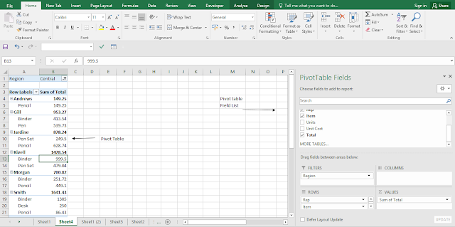A simple Pivot table set up

Download the sample data that we are going to deal with in this topic. click here

I think it is always better to convert the data source in excel table format first before arranging pivot table from the data source.
Excel will automatically update the pivot table in case a new data is introduced in the table.

In Pivot Table your source data should be in a rectangular database format. Informations that are available in the source should be of two types. 
Data (Say Total)
Data Category (Central Regions Total, even Smith performance total)

Default Pivot Tables

Instead of creating of pivot table from scratch one can select from some default styles provided in Excel. Under 'InsertTab' click 'Recommended Pivot Tables'. 

Excels provides some ready made Pivot Tables for your use. Intelligently it recognizes the data, one is dealing with.

• Select the entire Data range / click inside the range.
• Click Recommended Pivot Tables.

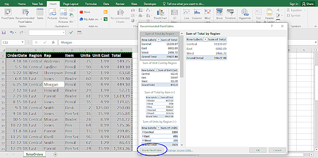Recommended Pivot Tables

From here even you can start your own Pivot Table by clicking Blank Pivot table button.
The table above contains 7 columns.

1. Order Date
2. Region
3. Representative (Rep)
4. Item
5. Units
6. Unit Cost
7. Total (Unit x Unit Cost)

Highlight any option and click Ok the pivot table will be placed in a new sheet with Pivot Table fields.
Even you can start your own pivot table from this option.
Say we select 'Sum of total of Region' from the list

Sum Total of Regions

By default the table is placed in a new sheet.You can see the accuracy of the table, Grand Total confirms the sum of Total column. 

Lets modify the pivot table at your discretion.

This is to remember that one should start with a query for the presentation. There are innumerable queries, we will discuss few in this respect. One should practice with his own data set.

Laying out Pivot table

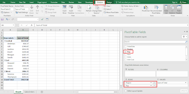
Fields in the 'Pivot Table Fields' window can be dragged in four spaces (Filter, Column, Row and Values). Say field 'Region' can be dragged in the Row area and field 'Total' can be dragged into the Value Space. Again if you want to remove any field from the above 4 spaces just drag out the field from the space. Or left click on the field on any of the 4 spaces, click 'Remove Field'.

Instance 1

Query: Presenting how Representatives performed in different regions.

• Click the check box relevant to Rep in Pivot Table Fields Task Pane.

 

A new tab 'Analyze' has been generated in the above ribbon. It is activated if we click anywhere inside the pivot table. As you can see in the above display a new field 'Rep' has been incorporated under Row option. 

Instance 2 

Query: Presenting how Representatives perform item wise in different regions.

• Click the check box associated with Item

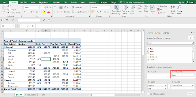
Lets again modify the presentation. Drag and drop the 'Item' in the Column field. We will see that the presentation will be much more concise, dynamic and meaningful.

Lets analyze the presentation a bit. Morgan in the Central region sold Binder, Pen set and Pencil to the tune of Rupees 251.72, 686.95 and 449.10 respectively totaling 1387.77. 
Revenue generated in the Central region from Binder is rupees 5762.63. Total revenue generated from Binder is Rupees 9577.65
 There is no sale of Desk in the Eastern Region and no sales of Pen Set in the Western Region.
So we see how a simple range of data evolves into a much  meaningful information.

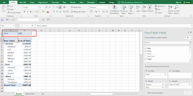
We can modify the presentation again. Remove the Rep from the Columns area and put the field in Filter area.

Item field is shifted at the top (Marked with Red). We are going to filter the pivot table according to item.
Pivot table displayed the consolidated figure of total sales generated as (All) is displayed above. 

Lets represent the region wise 'Pen Set' sales generated by representatives.

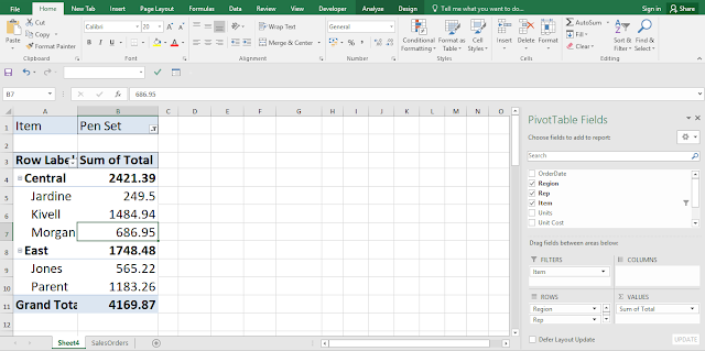
If we observe the previous display total Pen Set sales (4169.87) is still the same, but table represent it in a different manner.

You can select multiple items from the drop down box. 

Instance 3 

Query: Representation of Number of units sold item wise by different representatives in the 3 regions.

Pen set sales in different regions by representatives.

Explanations: 

• Item field has been placed under Filter area.
• Pivot table fields display window has been removed deliberately to fit the table.
• Total Pen set sales is same as before 4169.87
• No Pen set sales has been generated in Western Region
• Total sales generated by Kivell is 138 but in different dates that 42 & 96 that is why represented differently.
• Pen set sales in Central is 2421.39 & in East is 1748.48

Again with Multiple items say Pen & Pen Set the table is big. 





Explanations: 

• Units (B4 to L4) here represents consolidated sales figure of Pen & Pen set.

• Emphasis is on the Representatives whose performance is measured in respect of two items. That is why consolidated figure of Pen & Pen Set is shown.