Wednesday, October 30, 2019

Find & Replace | Replace

Replace

Replace is an important function in Excel.
May be it is convenient to alter the cell content where the number of cell is less, but when data is huge Replace function excels.

One can alter/change/remove the content of cells by use of Replace function.

It is located in 'Find & Select' function under Home tab.
Short Cut 'Ctrl+F.'


Find & Replace

Easy and simple format just 'Find What' and to 'Replace With'. 

Replace is an intelligent function to remove or delete any particular content of cells from the data sheet. 

Say we want to remove or delete the text 'Binder' from the datasheet. 
Just type 'Binder' in 'Find What' text box, and keep 'Replace with' text box blank. Press the button 'Replace All', it will just replace or delete all text 'Binder' from the data sheet and keep the cells blank as we didn't specify anything to fill in. 
Now the problem may arise that it will delete or replace the text 'Binder' from all cells but where there may be a text called 'Hard Binder' it will remove text 'Binder' and text 'Hard' will only be left in the cell. 

To overcome this problem
  • Click the 'Options<<' button.
  • Tick the box 'Match entire cell content'.
Now the replace function will ignore the text 'Hard Binder'.


Replace Format

It is an intelligent option to change the format of cells.
Say we want to make 'Binder' text into 'Bold' in all the cells where the content is 'Binder'.


  • Press Ctrl+F (Find & Replace Dialogue box pops up).
  • Activate Replace Tab.
  • Click 'Options > >' button.
  • Write 'Binder' in both the textbox (Find What & Replace With) since we are going to replace 'Binder' with 'Binder' just with different format.
  • Click 'Format' button relative to 'Replace with' (Extreme Left).
  • In the 'Replace Format' dialogue box.
  • Activate 'Font Tab', highlight 'Bold' under Font style.
  • Again Activate 'Fill' tab.
  • Click 'Fill Effects'.
  • Under Shading Style highlight any Variant.
  • Click Ok
replace format
  • Click 'Replace All'. 
All the 'Binder' text will be replaced with a special format you chosen.Under preview button one see the format that will be incorporated.
One can clear the selected format by clicking 'Format' button and Click 'Clear Format' option.

Sunday, October 27, 2019

Find & Replace | Find

Find

Find is an option in Excel with the help of which we are going to find anything in the data sheet/worksheet. 
Find is a search function inbuilt in Excel.
One simply needs to specify the search criterion. Excel will do the rest.
It is located in 'Find & Select' function under Home tab.
Short Cut 'Ctrl+F.'

Previous post's data sheet is used for demonstration.


find and replace
Find & Replace
find window
Find Window
How to find? 
Say we want to find 'Smith'. 
Type Smith in 'Find what' text box. 
If you press Find Next, you can view cells one at a time where content of the cell is Smith. In fact it is not the view, the cursor goes on making each Smith's cell active when you press Find Next.

If you press 'Find All' a separate window pops below where number of find can be seen with respective cell names.
And if you click each row in the window the cursor will move to the respective location in the sheet.

found
Results of Find

3 Cells found. 
Now where the results are located?
In the SalesOrders(2) sheet of Filter.xlsx file. 
And the respective cell numbers are C15, C21, C24.


Links has been created for each find. Cursor transforms into 'hand' when we hover the mouse cursor above each entry. If we click any entry excel makes the respective cell active in the corresponding data sheet. 

Here excel ignores upper case and lower case sensitivity.
Since we put 'smith' for search criterion but the contents are 'Smith'.


But interestingly excel accepts any blank space into consideration.
Say if we put smith with a blank space after h (by pressing space bar) excel will fail to find any. Since no cell contained with Smith has any blank space after h. Of course if any content of cell with smith is with a blank space after h, excel will find that cell.

Again excel can find any blank space 'only'. We put a blank space in the Find What text box (by pressing space bar once), and we know a cell with Smith has a blank space after h.
Excel can find that cell along with other cells where there are blank spaces.
Excel can find special characters. Say #, @,. etc

Even excel can find digits or alphabets in any content. Say we put 2 for search, and a date 10-12-2019 is there. Excel will take into consideration this date along with other content say 72,727 etc.

Again if we put '-2' for search, excel will find this date only with other dates where search criterion matches.

You can also use wild card characters like *,? for search criterion.
Type p*n to find string of characters say pen & pencil. 
Again type c*l to find central and pencil.

Use question mark ? to find a single character.
Put p?n to find pen. 
Put 4?9 to find 449.10.

Now if we want to find ? or * what will we put as a search criteria?
Put ~ (tilde) just above the tab key in keyboard.
~? or ~* to find ? and * respectively.

Advanced find options

Click 'Options>>' in the  Find & Replace window.

advanced find option
Advanced Option

In advanced option One can specify the sheet or workbook to search, by clicking at 'Within' combo box. 

One can specify the pattern of search say by row or column wise. If column wise is specified excel first reads the first column then the next and so on. In row wise search excel search rows one after another.

Lookin combo box specifies whether to search formulas also including text. And if one specifies text in the combo it ignores formulas. Say 2 is multiplied with the content of the cell G1 and the formula thereof would be G1*2. Now if we search G and specifies 'text' in the drop down combo it ignores the G in the formula cells. It may be handy. 

Now one can search contents of comments by specifying 'comments' in the look in combo box. Where in the search ignores all cell that are not commented.

Another important aspect of Find is, one can specify the area of the search in the worksheet. Say we need to search a telephone number within a column of telephone numbers. We can select the column only and search. Search results will be limited to the column only.


Match Case:

As it has been said that excel ignores uppercase and lowercase in case of ordinary search. But if we tick the check box associated with Match Case, excel will be very specific about its search. Excel will make the difference between SMITH & smith. If we search for 'smith' it won't find 'SMITH'.

Match Entire Cell contents:

If we tick the check box associated with 'Match Entire cell contents' excel will again be very specific about its search. In the ordinary scenario if we want to search for 'Binder' we can put the search criteria as 'bind'. We the box is ticked it won't find 'Binder' with search criteria 'bind'. It will consider those cells where entire search criteria matches.


Find Format:

We can search and find a particular format in the worksheet or workbook. Say we want to find all the 'bold' characters in the data sheet. 


find format
Find Format
  • Click 'Format' (as above).
  • Under 'Find Format' dialogue box click Font Tab. 
  • Under Font Style click or highlight Bold. 
  • Click Ok.
  • 'Find What' text box should remain empty because we are not searching any particular text or digit. We are simply searching the bold characters and digits in the sheet.
  • Click 'Find All'. 
  • Even you can search for colored cell, font style, italics, underlined etc. in this manner.

Thursday, October 24, 2019

Sort and Filter | Chapter 2 | Filter

Filter

To access Filter function click 'Sort & Filter' option under Home tab.
filter function

  Filter function is also available under  'Data' tab.

How to incorporate Filter function?
  • Click anywhere inside the source data where you want to incorporate Filter function.
  • Click Filter (as marked with Red above).
drop down arrow
Filter option enabled


We are going to use simple data sheet to understand Filter function.
Excel Table has default Filter option enabled.


Download the data sheets here.

We are going to understand filter function with the help of some examples. 

Instance 1


Filtering the data according to Central Region.
  • Click drop down arrow of Region cell (B1).
  • Uncheck '(Select All)'.
  • Check 'Central'.
  • Click Ok.


filtered data
Explanations: 
Drop down arrow of Region (B1 Cell) has been changed to a 'Filter' sign. It symbolizes that the column has been filtered. Again in respect of rows it can be seen that some rows has been hidden only. Original data is intact.
If you want to view the entire sheet without filter. 
  • Click the filter symbol on Region cell.
  • Check (Select All).

Instance 2

Lets filter out representative Smith's performance in the Central region.
  • Central Region to filter as above.
  • Click drop down arrow of Rep cell.
  • Uncheck 'Select All'.
  • Check 'Smith'
  • Click Ok
 Representative Smith's performance
Explanations:
Region and Representative column has been filtered as drop down arrow has been changed to a filter symbol. 
Now if we want to revert to the original view, then we have to remove filter from Rep first and then from Region. It is better to remove filter from the last filtered column first and then proceed accordingly.

Instance 3

Excel automatically recognizes date format.
It changes it filter box accordingly.


Lets find out the performances in Jan & Feb for 2019 only.

  • Click the drop down arrow Order Date cell.
  • Again Uncheck '(Select All)'.
  • Click the '+' button associated with 2019.
  • Check Jan & Feb.
  • Click Ok.
sales for Jan & Feb

Alternatively

Lets find out a different fashion for achieving the same result as above.
  • Click the drop down arrow in Order Date cell.
  • Guide the mouse pointer to 'Data Filters'.
  • Click 'Between'.
  • Check the radio button 'And' if not checked.
  • Put the start Date 1-01-2019.
  • Put the end Date 28-02-2019.
  • Click Ok.

custom auto filter
Custom auto filter dialogue box
  Explanations: 
  • Adjust dates by click the icon marked with Red circle.


Instance 4

Lets find out in respect of the item 'Binder' the representatives who failed to achieve triple digit sales figure.
  • Click the drop down arrow of 'Item' cell. 
  • Uncheck Select All.
  • Check Binder.
  • Click Ok.
  • Again click the drop down arrow of 'Total' cell.
  • Hover the mouse to option 'Number Filters'.
  • Click 'Less Than.......'
  • Put 100 (since any amount less than 100 is double digit figure ignoring decimal places of course).
  • Click Ok.


custom auto filter
Custom Auto Filter
Result as follows: 

sales less than 100

Slicers & Timeline can also be used to filter data. 

Monday, October 21, 2019

Sort and Filter | Chapter 1 | Custom sort

Sort & Filter

Meaning of Sort in Excel.
Rearrangement of rows on the basis of a content of a particular column.

sort and filter icon
Sort & Filter

Located under Home Tab 
By clicking the Sort & Filter Drop down arrow

sort type
Sort type


We are going to discuss with a data sheet. If required one can download here.

data sheet
DATA Sheet
There are immense opportunities for filtering and sorting. 

Excel automatically understands the sorting opportunity accordingly.
For instance when the active cell is under Date column the sorting field will change from 'Sort A to Z' or 'Sort Z to A' to 'Sort Oldest to Newest' or 'Sort Newest to Oldest'.


By default it is 'Sort A to Z' or 'Sort Z to A'.

How to sort?

  • Active any cell of the column on the basis of which you want to sort.
  • Click 'Sort & Filter'.
  • Sort A to Z or lowest to highest or newest to highest accordingly.
Excel effectively understands column headers. Excel won't include column headers such as Order Date, Region, Rep, Item etc as the item for sort.
Now if we delete the header row excel will sort the entire data as it cannot identify any header row as such.
Again in the above data sheet if we select the entire data (including header row) excel will sort according to date, since it is the first column in the data sheet. 


If we consider each row of the data as a 'Data Record' Excel will sort each data record on the basis of your choice. You can try this by coloring a data record with a specific color of your choice.


Custom Sort

Custom sort is interesting and I always prefer one to go with custom sort. May be it is complex.
levels under custom sort
Custom Sort window

In the case of the above data sheet Excel automatically finds the header row as you can see 'My data has headers' check box is checked. If there no header row then excel will sort column by column name say 'A', 'B' etc. Even one can de check the associated check box of 'My data has headers' and perform sort by column name.

Add Level is very interesting options in custom sort. Say, you want to first sort the data sheet by date (say Oldest to newest) and then by Region (say A to Z).

The sort window is somewhat as follows.
custom sort window

Click Ok
You can also shift levels up or down in multi column sort. 

Custom List

Custom List is another very important aspect of Custom Sort. 
For instance, in the case of the concerned data sheet if we want to sort the 'Item' in the order of Desk, Pen, Pencil, Pen Set, Binder.
That means neither A to Z nor Z to A, just an order of our own.
Under Order there is an option called Custom List.
Here we can find other orders that Excel Follows. Default lists cannot be deleted.

sort by custom order

Click Custom List

 
custom list

Write in the 'List Entries Text Box'
"Desk, Pen, Pencil, Pen Set, Binder" 
Alternatively first write Desk and press Enter then write Pen and press Enter and so on. As it is said 'Press Enter to separate list entries' in the window itself.
Click Add and the new series will be shifted to the left under Custom List window.
Then Click Ok.
This custom series will be highlighted in the custom sort window 'Order'.
This list will remain in the excel unless one deletes the same.

Friday, October 18, 2019

Fill Data | Chapter 3 | Fill Handle

Fill Handle


In the previous chapters we dealt with filling data in excel. In this chapter we will understand the shortcut method of feeding data in excel with Fill Handle or Cross Hair. Truly speaking most excel users are much comfortable with this approach. 
A very small length video.


Explanations: 
  • The plus '+' sign or cross hair is the Auto fill handle. 
  • After left click pressed and dragged, at the end of the selection another dialogue box emerges called 'Auto Fill options'. 
auto fill handle & Auto fill options

We will discuss each and every aspect of Auto Fill option box. Except Flash Fill already discussed in the immediate previous chapter. Click here.

Copy Cells: Only the cell content is copied by click and drag. Since the content is copied the relevant radio button is already checked.

Fill Formatting Only: Say at the above display if we check the radio button 'Fill Formatting Only', format of the source cell will be copied to other cells (The texts will be erased and formatting will be set in from the source cell).

Fill Without Formatting: Alternatively texts only be copied to other cells. No formatting will be transferred from source cell.

Since auto fill handle and option is an operational procedure it is better to understand the procedure with the help of a video.


Instances of auto fill
Some query for auto fill
Result as follows:
Left Click & Drag

Explanations: 
  • Instead of Click & Drag one can double click on the Fill Handle. Excel automatically fills the cells below it with the required data. In case of Fill Text, format is also copied along with the  content of the source cell. And with the Auto fill options box one can change the fill.
  • Double click wont work if there is no corresponding data that tells excel the extent of the fill. Here Formula column already been extended to 14th row so excel understands and assumes that the length of the fill may be up to 14th Row. Even if there is a blank row in between, excel will stop at the blank row. Say if 10th row is all through blank then excel will calculate up to 10th row.
  • Another trick - instant of Left Click and Drag what about Right Click and Drag of the Auto Fill handle?
Say in case of the date series as above if we Left Click and drag the Auto fill handle another window appears that has other options too. And when you click any options in the window excel will fill the column accordingly.


Disabling Auto Fill Handle & Options

By default the option is enabled but if any one wants to disable the option one can follow the steps below.
  • Click File Tab
  • Click Options
  • Click Advanced (Left Pane)
  • Check out 'Enable Fill Handle and Cell Drag & Drop'.


Tuesday, October 15, 2019

Fill Data | Chapter 2 | Series | Flash Fill

Series


We are going to understand in detail series function under 'Fill' option. 
Click Fill option under Home Tab.
Click Series 

Series Window

Lets understand different type of series with their respective videos.

Linear Type 

Lets understand linear series with the help of a video.

Explanations: When we select row space or column space excel automatically adjusts accordingly in 'Series in' option in series window. Observe the series window above.

 Growth Type

Each factor is multiplied by 'Step Value'.
Say, if Step Value is 2 and with 4 initial value the series will be 4,8,16,32....
Same as linear type we can limit the series by 'Stop Value'.

Date Type

 Lets understand Date Type series with the help of a simple video.


Autofill Type

Again we are going to understand the above type with a video.


Trend Type is similar to Autofill Type but it goes with any trend if there is any. Even it changes the source data to go with the trend.

Justify

Here justify option simply fits or spreads the text in multiple cells only.
In the below display the text is outside the cell.  The text is originally in cell G3. Now if we increase the cell width Justify won't help any.
text outside the cell

Instead of increasing the cell width if we click Justify under Fill function then the result will be as follows.

justify

Excel will justify a long text and spread it somewhat evenly through out the rows.
Excel after all is not a Word processor.👍👍👍

Flash Fill

Flash Fill is an interesting idea and it originated in Excel 2013.
It works well when the source data is absolutely consistent.
Any inconsistency results in error rather fallacy, and I personally do not advice to work on the basis of this when source data is large.

You are advised to observe this video. This is important.


Want to learn Across Worksheet function under Fill option. 
Click here.

Saturday, October 12, 2019

Fill Data | Chapter 1 | Across Worksheets

Fill button

Click the Fill button.

Fill details


auto fill handle
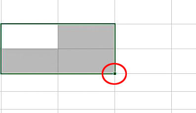
Cross Hair & White Cell of selection

Cross Hair/ Auto Fill Handle & White Cell

When you hover the mouse on the small Green solid square inside the Red Circle, mouse cursor transforms into '+' this plus sign is often called cross hair or auto fill handle. 
Now one can left click and drag the cross hair (with left mouse button pressed) and fill the vertical or horizontal cells with the data that has been selected. 
And white cell is the default active cell within the selection. 

You can deactivate auto fill handle option.
  • Click File.
  • Click Options.
  • Click 'Advanced'.
  • Check out 'Enable Fill handle and cell drag & drop.'
 
With the help of the following video we are going to understand Down, Right, Up and Left and Across Worksheet (Greyed above) function. And also observe how cross hair / auto fill handle is used.


Explanations:

Across Worksheets... function works after the working is carried on a single worksheet. The required sheets can be grouped and the workings can be transferred to the other sheets in the group. So when group is created Across Worksheets function is highlighted.

Instead if we create group of worksheets beforehand and any workings in a single sheet will be automatically posted into other sheets in the group. Say a text or a formula can be transferred. But format wont be transferred. Of course any change of format in a single sheet after the group creation will be contaminated to other worksheets in the group. Try it yourself.

Auto Fill selected Cells

  •  Select the blank cells where you want to fill with a.... say text 'excelintoexcel'.
  • After selection start writing excelintoexcel and you can see it is written on a cell (Default white) of the selection.
  • Press Ctrl+Enter
  • All the cells of the selection is filled with the text excelintoexcel.
Alternatively
You can achieve the same result by dragging with Cross Hair/Auto Fill Handle.

A simple video.


Alternatively
One can go with copy paste too.

Replacing the contents of the cell.


The best way to replace the content of a cell is to activate the cell and start writing the alternate or new content. The cell automatically fills with the new content but the format of the cell will remain and applies to the new entry. 

Editing the contents of the cell.

Best way to edit the contents of the cell is to replace with the new one. But if the content is textual say multiple line text.... then
  • DblClick on the cell and the cell will activate with the cursor starts blinking inside the cell. 
  • Guide the cursor where you want to edit with Navigation keys in the key board.
Alternatively.
  • Activate the cell.
  • Press F2 in the key board.
  • Guide the cursor where you want to edit with Navigation keys in the key board.
Alternatively you can also edit the content in the Formula Bar.

 Moving selection inside the sheet.

Sometime it happens that we want to move the workings in a different region in the sheet.
  • Select the content.
  • Hover the mouse over the perimeter of the selection.
  • Mouse cursor head is tagged with a Four Headed Arrow.
  • At that instance Press and Hold left mouse button start dragging the selection in the required region.
  • One can see that the content along with format is also shifted to the new region. 
  • Source region is left blank.


Some Data Entry Techniques 

After entering a data into a cell when we press enter in the keyboard the cell pointer automatically moves to the next cell down (by default). Now if you want to change this scenario. 

Under File tab > click Options > select Advanced 
Under Editing Option 
Uncheck the related check box under, 'After Pressing Enter, move selection' if one wants to disable this option. Or one can change the direction by selecting the drop down combo box.
Turning it off or on or change the direction is a matter of personal preference.
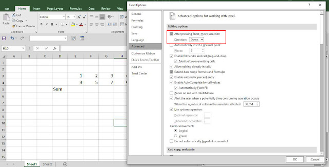
advanced tab
Marked with Red Box
Instead of pressing Enter after entering data in a cell one can use navigation keys to move to the next desired cell.

Selecting a range of input cells for entering data 

One can select a range of cells where the data entry is to be performed. After entering in the default white cell (of selection) if one presses Enter the cell pointer moves to the next cell inside the selection. You can skip a cell by simply pressing Enter again instead of entering anything in the cell. You can revert back to the previous cell by pressing Shift+Enter. This is to remember the cell pointer will remain inside the selection.

Entering decimal points automatically

If one is going to deal with lots of numbers with decimal places. Excel provides an easy approach to handle the situation.
If one specifies 2 decimal places and enters 2587 then excel interprets this entry as 25.87. Very easy and interesting.
By default this option is not enabled. 

For enabling it.
  • Under/Click File Tab.
  • Click Option.
  • Click Advanced.
  • Tick the check box associated with 'Automatically Insert a decimal point'

Automate data entry with auto complete feature.

A very useful feature of Excel. 
Easily you can enter same text in multiple cells.
  • The cells should lie in the same column where the entry is already been made.
  • There should not be any blank cells in between new entry and previous entry. There could be other entry but no blank cells. 
  • The feature takes into account the lower case or upper case too.
In the new cell if we start typing only the first few characters or alphabets of the text (previously written) excel automatically recognizes your try and give you an option to fill the cell with the previous entry. By pressing enter one can enter the previous entry in the new cell.

It enhances your accuracy of posting. You don't have to misspell.

Say when you enter the text 'excelintoexcel' excel remembers it.
Then when you start typing ex.. etc in the second entry excel provides you an option to fill the cell with 'excelintoexcel'.

You can disable this option of excel 
  • Click File tab.
  • Click Options.
  • Click Advanced.
  • Check out the 'Enable Auto Complete for Cell Values'.

Thursday, October 10, 2019

Pivot Table | Chapter 7| Calculated Field Calculated Item

Calculated Field And Calculated Item

Creating Calculated Field and Calculated Item is bit confusing sometimes. 

We deal with Calculated Field and Calculated Item once the Pivot Table is created. 

Download the sheet used with calculation.....Here

Calculated Field - A new field created from other fields in the Pivot table. Simply speaking a column is calculated from other columns in Pivot table. After creation it resides in the value area of the pivot table. One cannot shift this field to other areas. Alternatively and much easier is to create a column and add the same to the Pivot Table. But when we deal with any external database, Calculated Field is handy and only option left.

Calculated Item - Similarly a new row is created instead of column with the help of Calculated Item option.This new row resides in the Column area, Filter area and Rows area in the pivot table. And it cannot resides in the value area of the Pivot Table.

The formula we use to create the Calculated Field and Calculated Item is not the standard excel formula. Of course the math and logic is same. 

We will understand both with the help of a video.


Explanations:
  • After ungrouping the OrderDate it is advisable to select the region's cell (say central) before writing the formula in case of Calculated Item. (Though it is not full proof but I find it convenient)
Some important tips on Pivot Table
Pivot Table has some limitations, it is flexible enough but you cannot add new rows or columns or enter formulas within the Pivot Table. It is true you can enter column or row with the help of Calculated Field & Calculated Item.
                     Again if one wants to manipulate a Pivot Table data one can copy the same and paste else where to manipulate. When Pivot table is pasted else where it detaches itself from the Excel Table. Here Clipboard copying is the best option. 
And copied information is not pivot table and it is no longer linked to the source data.


Monday, October 7, 2019

pivot table | Chapter 6 | multiple sheet pivot table

Today in this chapter we are going to understand how to incorporate multiple sheet's data into a pivot table.

We have already created tables with the data of respective sheets.
Order Date data will bind the three sheets together and acts as a primary key in Database structure.

Order Date with Total

Order Date with Region

Order Date with Representatives

Table names are as follows
Table_Region for region
Table_Rep for representatives
Table_Total for Unit and Total column

Download the worksheet here
 
Relationships Diagram under 'Manage Data Model'

We are going to understand the entire procedure with the help of a video. 


Explanations:
Some time the relationship needs to be deleted.
Steps:
  • Under the Data Tab.
  • Click Manage Data Model.
  • Right click on the tab and click Delete.
 
deleting relationship

Saturday, October 5, 2019

pivot table | Chapter 5 | frequency distribution

we are going to understand how to deal with frequency distribution in pivot table. For reference we are going to use the table below. 

 excel data table
Download the table & working here

In simple word we are going to create some range to understand how different figures under the Total column fits in the different ranges. It is called 'Frequency Distribution'. This type of analysis is very useful. 

Steps:
  • Click inside the Data Table.
  • Under the Insert Tab click Pivot Table.
  • Select the table range if not selected.
  • Highlight the radio button for New Worksheet.
pivot table creation window

  • click ok.
  • Drag the Total column under Values Area. 
  • Left Click on 'Sum of Total' (Total Field) under Value Area.
  • Navigate down to 'Value Field Settings'.
  • Change the Value Field to 'Count'. 
  • Again drag the Total field to Row area.


piovt table with count value
  • Left Click inside the Pivot table  on any Total Figure.
  • Under Analyze Tab click 'Group Selection'.

grouping window
  • Starting & Ending figures are already incorporated, based on Highest and lowest. 'By' sets the distribution range. We can change it. But here we will proceed with 100 as default. 
  • Click Ok
pivot table with range
Explanations: 
Range difference is 100. Count column states the occurrence of different 'Total' values within different ranges. 
Say between 519.96 to 619.96 there is only one occurrence. Check Table, i,e, Gill's performance under Central region 539.73 '

Wednesday, October 2, 2019

Pivot Table | Chapter 4 | Grouping Ungrouping

Grouping and un-grouping with pivot table data. 


Grouping Ungrouping in Pivot Table
Grouping & Ungrouping Buttons

excel data table

Download the datasheet that we are going to use for demonstration in this post.

basic pivot table from the datasheet
Basic Pivot Table from the Datasheet
Explanation:
  • Region field is placed on rows
  • Rep (Representatives) are placed on column.
  • Value total is displayed.
Now lets introduce Order Date On rows.


order date grouped
Order date Grouped
Explanations: 
  • As usual two group fields has generated - 'Quarters' and 'Years'.
  • Region, Years, Quarters and Order dates are incorporated into Rows area.
Lets ungroup years. 
  •  Select any year cell.
  •  Click Ungroup under Analyze tab
ungrouped dates
Ungrouped into basic order dates
Explanations: 
  • Years has been ungrouped into basic ordering dates.

Now we are going to group dates as per Qtrs and Months and years.

  • Select any cell with dates.
  • Click the button Group Selection.
  • Check the relevant date range. 
  • Highlight Months, Quarters, Years.
  • Ignored Days else one can highlight Days too. 
 
grouping window
Grouping window


grouped and disintegrated
Grouped
Explanations:

  • Negative buttons can be clicked  to integrate the rows.

We can create our own group with existing groups. 

One of the most useful features of Pivot table is the ability to create groups

grouping in pivot table
Above is the default table. Lets Create Group 1 with Central and East Region. 
  • Select Central and East Region (Including years)
  • Under Analyze Tab click 'Group Selection'.
creating own group
Explanations:
  •  New Group 1 emerges. 
  • One can ungroup this group.

Timeline 

 Instead of adjusting filters to deal with dates, one can use Timeline.
Timeline is a filter option that one can use to zoom a particular date/time period in the pivot table. It is handy.
Click inside the pivot table > Under the Analyze tab click Time line

In the instance Timeline will deal with 'Order Date'.
pivot table timeline
Explanations: 
  • Display name (Order Date) can be changed. Change the Time Line Caption (Ribbon Left).
  • The Timeline window comprises of two sliders one (colored) to highlight the zoom option that is particular month, year, qtr etc, and another slider helps to navigate the zoom bar.
  • In the Timeline window there is a zoom bar, here by default it is zoomed in months. If one clicks on the sliding bar at a particular point of the month the Pivot Table will change accordingly.
  • Again Month option can be changed to Qtrs and so on.
  • You can change the Timeline styles.
  • One can reset the Timeline by clicking at the top right corner icon.