Excel Table 4 | slicers

                                   SLICERS 

 

A table can be filtered by Slicers. They are highly appealing. 

Though not flexible enough. And it consumes lots of space on the data sheet. When space is a problem one can cut and paste those slicers in a different sheet. It will work fine.

It is good when data in the sheet is minimum. But when data is large slicers don't get enough space to fit in. Slicer perhaps not appropriate when dealing with numeric data.

Slicer is located under Design Tab. Click inside the table and Design tab gets activated. 'Insert Slicer' is an icon under the Design Tab.

Datasheet download




  Lets click Insert Slicer

Insert Slicer Icon

The dialogue box above in the display lists all the columns of the table under consideration.
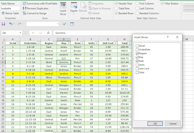
If we check mark all the columns that are listed in the box. Your excel sheet is somewhat as below.

So we don't need all the slicers, lets deal with limited slicers, we deleted slicers other than Region, Representative (Rep) & Units.

 Lets check all the relevant associated box. And click Ok. 

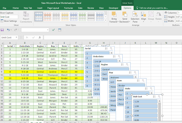
All the slicers that are required for sorting are placed in the data sheet.Slicers are arranged in the sheet by dragging.

If we look closely another tab generates above in the ribbon that is 'Options'. This tab helps us to deal with slicers as well as the  table.

If we go by logic these three slicers are selected because all the elements of the respective slicers have duplicates. Say more than one central, east and west record in the table. So duplicate value may be a basis for selection of slicers. Slicers are not case sensitive, 'EAST' & 'east' are same for slicers. 

Lets see how slicers work.

Explanations:

• Slicers can be stretched. Slicer can be highlighted by clicking inside the slicer space.
• Data are to be reset by clicking 'Clear Filter' icon on the right top in the slicers window. Even reset can be done by clicking the filter drop down arrow on the headers in the table itself.
• You can start sorting with any slicer window. Say, we can start sorting with 'Item' first then with Representatives and then with Region.
• When you press a data button inside a slicer window other data buttons are greyed out in that window. And other slicers are automatically adjusted with their data. Data buttons in other slicers that are not greyed out signifies sorting is possible with that data further.
• There can be enumerable combination.
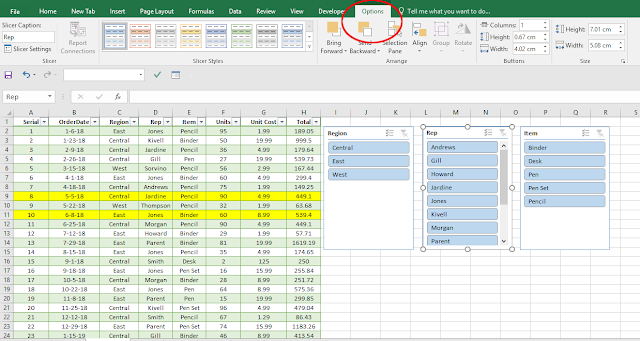
• With the Slicers Styles (under Option Tab) you can change the appearance of the slicer.  
• You can cut paste those slicers in a new window and those will work fine.

Multiple Selection option in Slicers

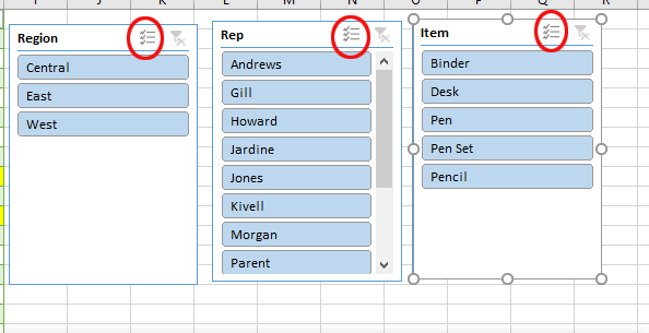Multiple Selection

Multiple selection option of slicers is marked with Red circles. Another thing to be noted 'Item' named slicer is highlighted. As 8 circle is surrounding the slicer. These circles or zeros can be dragged to resize the respective slicer. 


When the Multiple Selection option is activated (by clicking) one can select multiple data in the slicer. But interestingly the data button that we click, data hide itself from the table. Say with Multiple Selection option activated when one click 'Central' only 'Central' related data will be hidden in the table. After clicking 'Central' if we again click 'East' there will be only 'West' data available in the table. 
This is just the opposite when Multiple Selection option is not activated. When not activated if we click a data button in the slicer only that data is shown in the table and others are hidden. Say if we click 'East' only East related data will be shown in the table and others are hidden.
So learn this trick before applying slicers  in a huge and important data sheet. 

Slicer Settings 

Slicer setting can be activated by right click on the slicer and click slicer setting.

Again one can activate setting by clicking Slicer Setting button under Options tab.

Slicer Setting

One can change the caption of the slicer. Slicer by default takes the column name from the table. But by renaming the caption text one can change the displayed text in the slicer. 
Even we can hide the display name by uncheck the Display Header check box.
Every slicer has a name that are displayed in the 'Name Box' (at the extreme top left of the data sheet where also cell names are displayed). As we can change the name of a cell we can also change the name of slicer by changing the Name in the setting.

Slicer Size 

 

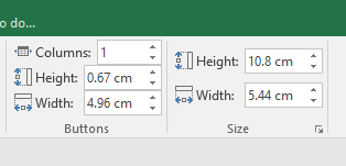
Slicer size and buttons size can be changed by using Height & Width buttons respectively. 
By default buttons are displayed in the slicer in columns. Column settings can be changed. Previously in all display in this post slicers are single columned.

Two columned slicer