Sort and Filter | Chapter 2 | Filter

Filter

To access Filter function click 'Sort & Filter' option under Home tab.

  Filter function is also available under  'Data' tab.

How to incorporate Filter function?

• Click anywhere inside the source data where you want to incorporate Filter function.
• Click Filter (as marked with Red above).

Filter option enabled

We are going to use simple data sheet to understand Filter function.
Excel Table has default Filter option enabled.


Download the data sheets here.

We are going to understand filter function with the help of some examples. 

Instance 1

Filtering the data according to Central Region.

• Click drop down arrow of Region cell (B1).
• Uncheck '(Select All)'.
• Check 'Central'.
• Click Ok.

Explanations: 
Drop down arrow of Region (B1 Cell) has been changed to a 'Filter' sign. It symbolizes that the column has been filtered. Again in respect of rows it can be seen that some rows has been hidden only. Original data is intact.
If you want to view the entire sheet without filter. 

• Click the filter symbol on Region cell.
• Check (Select All).

Instance 2

Lets filter out representative Smith's performance in the Central region.

• Central Region to filter as above.
• Click drop down arrow of Rep cell.
• Uncheck 'Select All'.
• Check 'Smith'
• Click Ok

 

Explanations:
Region and Representative column has been filtered as drop down arrow has been changed to a filter symbol. 
Now if we want to revert to the original view, then we have to remove filter from Rep first and then from Region. It is better to remove filter from the last filtered column first and then proceed accordingly.

Instance 3

Excel automatically recognizes date format.

It changes it filter box accordingly.

Lets find out the performances in Jan & Feb for 2019 only.

• Click the drop down arrow Order Date cell.
• Again Uncheck '(Select All)'.
• Click the '+' button associated with 2019.
• Check Jan & Feb.
• Click Ok.

Alternatively

Lets find out a different fashion for achieving the same result as above.

• Click the drop down arrow in Order Date cell.
• Guide the mouse pointer to 'Data Filters'.
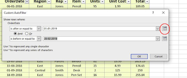
• Click 'Between'.
• Check the radio button 'And' if not checked.
• Put the start Date 1-01-2019.
• Put the end Date 28-02-2019.
• Click Ok.

Custom auto filter dialogue box

  Explanations: 

• Adjust dates by click the icon marked with Red circle.

 

Instance 4

Lets find out in respect of the item 'Binder' the representatives who failed to achieve triple digit sales figure.

• Click the drop down arrow of 'Item' cell. 
• Uncheck Select All.
• Check Binder.
• Click Ok.
• Again click the drop down arrow of 'Total' cell.
• Hover the mouse to option 'Number Filters'.
• Click 'Less Than.......'
• Put 100 (since any amount less than 100 is double digit figure ignoring decimal places of course).
• Click Ok.

  

Custom Auto Filter

Result as follows: 

Slicers & Timeline can also be used to filter data.