Formula | Chapter 5 | Workday

Workday formula

A very simple formula and much usage too.

In simple terms this formula ascertains a date (past or future), may be a due date.

Syntax

 =Workday(start_date, days, [holidays])

 start_date= A date to represents the start date.

days= A number of working days other than holidays and weekends. Negative days denotes past date.

Above two parameters are required.

holidays = An optional list of one or more dates to exclude from working days.

Formula Workday ILL1

Explanations:

Manual calculations has been made to understand the essence of the formula. Two respective dates in bold (colored) representing two formulas. For the sake of understanding two formulas also written below the dates. I request all to redo the process.

Workday.int Formula

A simple formula with usage.
It determines a date (future or past). May be a due date. 
Very much similar to workday formula.
Syntax
=workday.int(start_date, days, [weekend],[holidays])
start_date = A date.
days = numeric value.
start_date and days are required.
weekend = (1-17)This parameter signifies the counting option. Ordinarily weekend comprises of 'Saturday' and 'Sunday'. Default parameter.
But if one wants to vary the calculation of weekend. They can specify.

1. Saturday, Sunday (Default and can be omitted)
2. Sunday, Monday.



3. Monday, Tuesday. 
4. Tuesday, Wednesday.
5. Wednesday, Thursday.
6. Thursday, Friday.
7. Friday, Saturday.
11,12,13,14,15,16,17
Sunday, Monday, Tuesday, Wednesday, Thursday, Friday, Saturday,
respectively.

Formula Workday.int ILL2

'Year' Formula

This function/formula returns the year corresponding to a date.

Syntax
=Year(serial_number)
Lets use ILL2
And use the date in cell C4
=Year(C4)
Returns 2020.

'Yearfrac' Formula

This function calculates the number of whole days between two dates. It returns numeric values with fraction where needed.

Syntax

=yearfrac(start_date, end_date, basis)

start_date= A date. (future or past)

end_date= A date. (future or past) 

basis = 0,1,2,3,4

0 - US (NASD) 30/360 (no need to specify can be omitted)

1 - Actual/actual

2 - Actual / 360

3 - Actual / 365

4 - European 30 / 360

Formula yearfrac ILL3

Explanations:

In the ILL1 1.01666667 is the result of the formula =yearfrac(E6, E7, 2) - Basis 2 that signifies Actual / 360.

 

 


 

Formula | Chapter 4 | Time

'TIME' formula

This formula returns the decimal number of time and return value varies from 0 to .99988426.

Syntax
=Time(Hour, Minute, Second)

Here Hour, Minute and Second is represented by 0 to 32767.
In case of hour, if any value is greater than 23 will be divided by 24 and remainder will be treated as hour value. 
Similarly if any value is greater than 59 in case of Minute the same shall be converted into hour and minute.
Again if any value is greater than 59 in case of Second the same shall be converted into hours, minutes and seconds.

Time Formula ILL1

Explanations: 
Go through the above illustration and try it yourself. 
This illustration is self explanatory. 

'TimeValue' Formula

 This formula converts a text to a serial number for time, ranging from 0 to .99998426.

Syntax

=Timevalue(text)

Say

=Timevalue("12:00:45 am")

returns 0.000520833

Instead if we replace am with pm

formula returns 0.500520833

'Today' Formula

This formula returns the current date. Actually it picks up the system date.

A widely used formula.

Syntax

=Today()

Returns the current date - say '28-03-2020'.

 'Weekday' Formula

This formula returns the day of the week corresponding to certain date.
Syntax
=Weekday(serial number, return type)
We can proceed without specifying the return type.
say, 'Weekday(Date)'
The formula returns 1-7 integer only.
It simply specify the day of the date in a week. And return type parameter specify the counting pattern.
Counting syntax (1,2,3,11,12,13,14,15,16,17)
1 - Default 1(Sunday) to 7(Saturday)
2 - 1(Monday) to 7(Sunday)
3 - 0(Monday) to 6(Sunday)
11 - 1(Monday) to 7(Sunday)
12 - 1(Tuesday) to 7(Monday)
13 - 1(Wednesday) to 7(Tuesday)
14 - 1(Thursday) to 7(Wednesday)
15 - 1(Friday) to 7 (Thursday)
16 - 1(Saturday) to 7(Friday)
17 - 1(Sunday) to 7(Saturday)
 

Formula 'Weekday' ILL1

Explanations: 

Column C only represents the basic formula or default formula.
For instance, 15-03-2020 falls on Sunday (consult calendar). And formula returns 1.
Say, the formula with date 21-03-2020 returns 7. Calculating 7 from 15th March and ends on 21-03-2020 (inclusive).
Now if we deviate the calculation from the default calculation.
=Weekday(serial number, return type)
'return type' specifies different calculation option.
Options are specified in 2nd row. And they are 1,2,3,11........17.

 'Weeknum' Formula

This formula returns the week number of a specific date.
The formula returns 1-52 or 53. Since a year is comprised of 52 weeks.
It is bit similar to 'Weekday' function.
Syntax
=Weeknum(serial number, return type)
Return type (optional) determines on which day the week begins.

 

Formula 'Weeknum' ILL2

Explanations:
Return type here denotes numeric values 1,2,11,12.....21.
For instance numeric value 15 denotes..... week counting starts from 'Friday'. Hence the result varies.

Formula | Chapter 3 | Month

'MONTH' formula

This formula returns the month 1-12. This formula simply picks the month in the date.

Syntax
=Month(Serial_number)
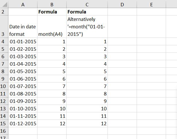
Observe the illustration below.

Month Formula ILL 1

Explanation:

Under alternative method the formula picks the month from a text string. 

'NETWORKDAYS' formula

This formula calculate working days between two dates.

Syntax

=Networkdays(Start_date, End_date, holidays)

Observe the illustration below

Networkdays ILL2

Explanation: 
The formula above returns 262 days. (Try It) 

NETWORKDAYS.INTL formula

This formula is a bit modification of the 'networkdays' formula.

Extra parameter weekend is added.

Syntax

=Networkdays.intl(Start_date, End_date, weekend, holidays)

while writing formula weekend can be picked up from the auto drop down box. 

Networkdays.intl ILL3

Explanation: 
The above formula returns 314 days. (Try it) 

'NOW'  formula

This formula returns the current date & time.

It actually accepts system's date and time. This is widely used formula. It usually don't require any parameter from user.

Syntax

=Now()

This formula above returns the current date and time.

(Since I am writing this blog at the below mentioned date and time.)

01-12-2019 10:23.

(Things to remember: This formula update itself automatically)

There are some variations available to the above formula.

Say (01-12-2019 as base date)

we calculate the 7th day date from the present base date,

formula is 

=Now()+7

Returns 8-12-2019 10:23

 =Now()-2.25 

Returns date 2 days 6 hrs ago. Since .25 represents a qtr. Each qtr comprises of 6 hrs in a day.

 'SECOND' formula

This formula returns the 'second' ranging from 0-59.

Syntax

=Second(serial_number)

Second ILL4

Formula | Chapter 2 | Edate

'EDATE' formula

Edate is used to calculate due date or maturity date.
Syntax

=Edate(start_date, months)
start_date: denotes a date in date format.
months: denotes tenure of months of maturity.
We can quote this formula in different ways.
Say, we are going to calculate 12 months maturity.
A3 cell has date value 25-11-2018 (should be in a date format).
so the syntax is =Edate(A3,12)
Returns: 25-11-2019 (date of maturity).
Alternatively the syntax is
=Edate(Date(2018,11,25),12)
Returns the same value 25-11-2019 (date of maturity)

'EOMONTH' formula

It returns the serial number of the last day of the month before or after a specified number of months.

Syntax

=Eomonth(start_date, months)

start_date: denotes a date in date format.
months: denotes tenure of months of maturity.
We can quote this formula in different ways.
Say, we are going to calculate 12 months date.
A3 cell has date value 25-11-2018 (should be in a date format).
so the syntax is =Edate(A3,12)
Returns: 30-11-2019 (date of maturity).
Alternatively the syntax is
=Edate(Date(2018,11,25),12)
Returns the same value 30-11-2019 (date of maturity)

'HOUR' formula

Returns the hour of a time value, and the result varies between 0 to 24 only (whole number only....no 18.25). This formula works with decimal places. Say, in case of 1.25 it ignores 1 and works with .25 only.

Syntax 

=Hour(serial_no)

For instance

=Hour(1.25) 

returns 6

Again

=Hour(.25) 

returns 6

Actually .25 of 24 is 6........... (25% of 24 is 6)

 

ILL 1

Explanation:
Observe the ILL 1 carefully.

'ISOWEEKNUM' formula 

Returns the week number for the given date.

Syntax

=ISOWEEKNUM(date)

For instance

Cell A3 has date value  1-1-2019 in date format.

=ISOWEEKNUM(A3)

Returns 1i,e first week of the year 2019.

In case of  7-01-2019 formula returns 2.

'MINUTE' formula

The formula returns the minute of a time value. Minute is represented as integer, ranging from 0-59.

The formula accepts decimal places. No whole number.

Representing percentage.

Syntax

=MINUTE(serial_number)

For instance

=MINUTE("12:35 PM")

Returns 35

 

 

Formula | Chapter 1 | Date & Time

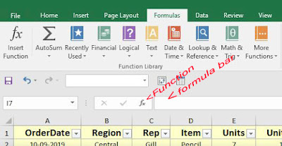
Formulas can be accessed by clicking at the 'Formulas' tab. 

Function key and 'Insert function' button serves the same purpose. 

'Formula bar' keep track of your formula. Not only formula, what you write in a cell is highlighted in the formula bar. 

When we click Insert Function / Function, Insert Function window pops open.

Insert Function Window

All type of formula resides in 'Insert Function' window. 
And if we click select a category combo box we can find the category of formula in excel.

Date & Time 

Interestingly Excel stores dates as sequential serial numbers.

And 1st January 1900 is the base year, and the serial is 1.

Accordingly, 1st January 2008 has a serial number 39448 since 1st January 2008 is 39447 days after 1st January 1900.

'Date' formula

Returns the number that represents the date in Microsoft Excel.

Syntax

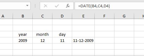
=Date(year, month, day)

Example

Date(2019,03,23).

Returns 23-03-2019.

Date function

 'Datevalue' formula

Converts the stored date into serial number.

Syntax

=DateValue("text")

Example

Date("1-1-2008")

Returns 39448

This function is mostly useful where worksheet contains dates in text format.

'Day' formula

Returns the day value from 1-31. And it calculates accordingly.

Syntax

=Day(serial_number)

Example

Day(100)

Returns 9
In fact representing 10th April. 

'Days' formula 

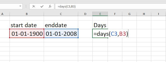
Calculates number of days from a base date. It can calculate backward too. Again the base date should not be later than 1-1-1900. 

Syntax

=Days(end_date, start_date)

Days360 formula 

Us or European method of approximation of days calculation from a base date.
Syntax
=Days360(start_date, end_date, method)
There are two methods
False=US method of approximation of 30 days.
True= European method.

Formula | Auto Sum | Deduct | Multiply | Divide

This is the first dedicated post on Excel Formula.
To access formulas click Formulas tab.
Even we can start with formula under Home Tab too.

Under Home Tab

Excel is always formula ready. One can start dealing with formula at any space. 

Things to remember

• Formula always starts with =
• While writing formula ignore upper case or lower case criteria, just start typing. 
• Instead of typing the cell values while writing formula one can link or denote the corresponding cell by clicking at the cell. Say, want to multiply F2 to G2, only type = and then click at F2 cell then type * lastly link G2 by clicking at G2 cell. Simple......

Lets start

Sum 

How to sum up cells with values?
Formula Syntax
=SUM(B3:B14)
(B3 to B14 cells are just imaginary)

Alternatively

=B3+B4+B5+B6.......................so on
Result will be same as before

For instance, we are going to sum up the values of cells F3 to F13
and display the summation at F14.

• Just select the cells F3 to F114.
• Under Home tab click 'Auto Sum'.

Excel will automatically make the sum of cells F3 to F13 and display the resultant figure at F14.

Alternatively
  

• At F14 cell start writing the formula as =sum(
• At this instance just select the F3 to F14 cells altogether.
• Close the bracket.
• Press Enter.

 

Deduct

Say we are going to deduct the cell value F13 from F14 cell value.
Very simple logic.
Write the formula
=F13-F14

Again
We are going to deduct 100 from cell F13 Value.
=F13-100

Multiply

In excel or precisely computer recognize * asterisk as a sign of multiplication.

Say, we want to multiply cell value F13 with G13 and display the result in H13.

At H13 cell write the formula 

=F13*G13

Division

Excel as well as Computer recognizes division with the sign '/'.

Say dividing  F3 cell with F2 cell.

Syntax is 

=F3/F2

Very simple logic.

Auto sum function is always very handy in all instance.

If we observe carefully it combines all function at once.

Observe the ILL 1 below.

ILL1

 

Explanation: 
Auto Sum function combines all.

Go to | last cell | visible cells only

Last Cell

Last cell denotes the cell that contains data and/or formatting.
Even one deletes the data and/or formatting of the cell, Last Cell function identifies that cell. 

Last Cell

Procedure

• Click any where in the sheet.
• Press Ctrl+G and click 'Special..' or Click 'Find & Select' under Home Tab and click 'Go to Special...'.
• Tick the Radio button associated with 'Last Cell' function.
• Click Ok.

Visible Cells Only

'Visible Cells Only' function identifies those cells that are visible in a range. It helps to identify the filtered rows or columns when filters are enabled in a sheet. 

Even it helps to identify any hidden row or column in the sheet.

It is useful.

Conditional Formats

'Conditional Formats' function identifies the cells with conditional format embedded.

Data Validation

Data validation function identifies cells with data validation embedded. Further sub categorized as 'All' and 'Same'.